
Fractal Art (AoC 2017, Day 21)
Table of Contents
- A Little Background (feel free to skip it)
- The Problem
- Brute-Force: The Naïve Approach
- $O(C^k)$, and how to Observe it
- Brute-Force 2: Concurrent Boogaloo
- Brute-Force 3: DP Rises
- Independent Evolution and Separable Elements
- Wrapping Up
A Little Background
I really like programming. Just coding for the sake of doing so is something I truly enjoy. I know that a large amount of people in the IT industry share this feeling, or at least they might have when they first got into this field. But as a doctoral ML researcher, I don’t have to deal with the downsides of industry programming, such as working with the unmaintainable clusterfuck of a codebase an intern wrote before I was hired or trying to explain to a PM why it’s taken 3 weeks to display the user’s birthday date on the setting page. My code is my domain, and I am free to develop it as I see fit or to burn it down and rebuild it from its ashes at my discretion; all my supervisors care about is that the error metrics go down and that the inference time goes Brrr.
However, being an ML researcher means the scope of technologies I can use is pretty narrow, especially when it comes to programming languages. Sure, I could write my own kernels in CUDA C++, or perhaps delve into Julia for some multiple-dispatch array programming with JIT compilation. However, I am not capable of iterating over model configurations and algorithms at the pace my job requires in C++ (skill-issued much?), and honestly speaking Julia does not provide a big-enough improvement in model performance w.r.t. Python to justify losing access to the data pre-processing, parameter tuning, and visualization stacks I rely on.
This does not mean I am stuck with the standard at every step; in fact, I use JAX/Keras because of its functional and JIT compilation APIs, even if most authors in the literature implement their papers using PyTorch. However, every deviation from the convention requires an investment in time, which in my case has been having to re-implement the models I could’ve just grabbed from the public repos. This is time for which I am getting paid, and there are deadlines I have to meet, so going against the current at every step is just plain irresponsible.
Now, don’t get me wrong: I really like programming in Python, and I enjoy my job. Nevertheless, I understand the reason I am getting paid to do something is because I cannot just quit whenever I get bored with repetitive tasks or lose interest on the topic I’m working with. Therefore, to nurture and preserve my love for programming, I mix my daily tasks with coding exercises in languages I would not be able to use in my daily job.
This is where Advent of Code (AoC)comes into play: a yearly set of 25 themed puzzles, increasing in complexity as Christmas gets closer, solvable in any programming language (and I really mean any) or even by hand. Since answers are requested as a number or a string, AoC does not coerce you into a specific algorithm or data structure. However, AoC puzzles have the particularity of being 2-fold, where the second part usually becomes unfeasible in reasonable time/memory if it is not approached cleverly. This allows for rather riveting optimizations and creative personal challenges. AoC draws a truly passionate community of developers, and this write-up is my first attempt at becoming an active part of it.
There is nothing inherently different about the problem in this post. However, this was the first time I felt all the techniques I had to learn while solving AoC questions came naturally to me as I was reading the question. I will first go through the problem structure, the naïve solution, the problems with it, and the optimization steps I took to reach my current best. Keep in mind I implemented my solution in Go which, even if compiled, relies on a runtime with a garbage collector, so I am sure further optimizations can be done by using a manually managed language like Zig or Rust.
The Problem
The full description can be found here. Picture a square grid $\left(N \times N\right)$ containing one of two ASCII characters, namely - (0 or off) and # (1 or on), and starting as:
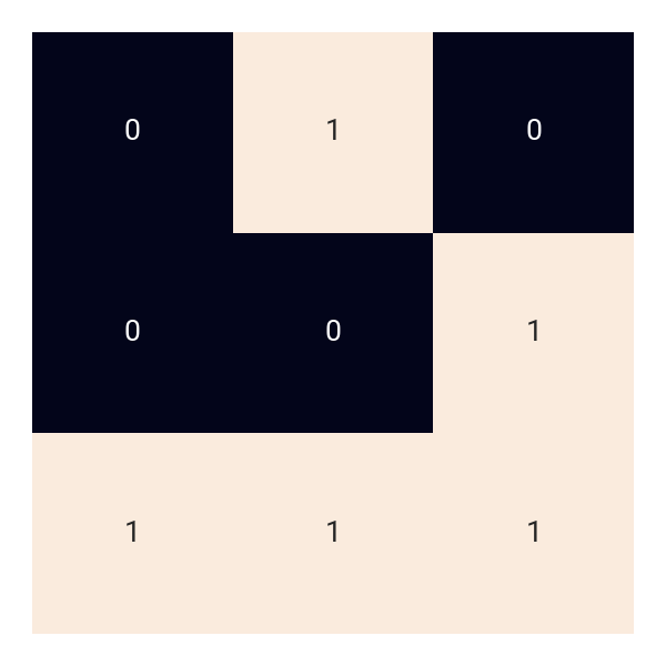
We’re told that this grid will evolve by applying one of two conditional procedures:
- If the size of the grid is evenly divisible by 2, break it up into 2x2 squares and convert each 2x2 square into a 3x3 square by following the corresponding enhancement rule.
- Otherwise, the size is evenly divisible by 3; break the grid up into 3x3 squares, and convert each 3x3 square into a 4x4 square by following the corresponding enhancement rule.
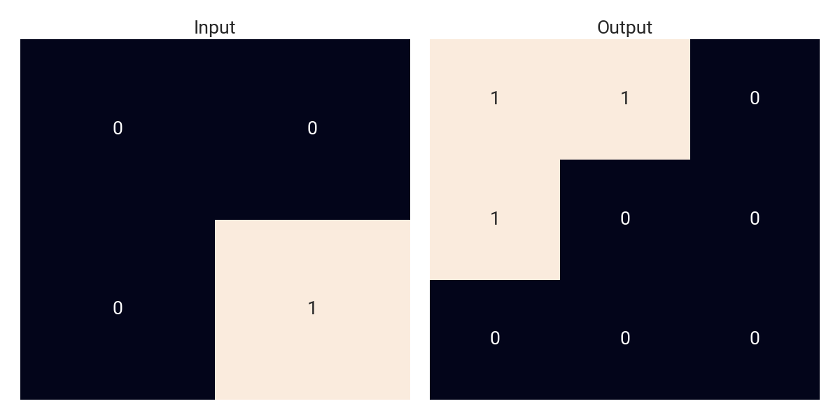
The aforementioned rules are passed to us as an input of the form
../.# => ##./#../...
.#./..#/### => #..#/..../..../#..#
Patterns are flattened and rows are separated using /, so the above rule-set describes the following transformations:
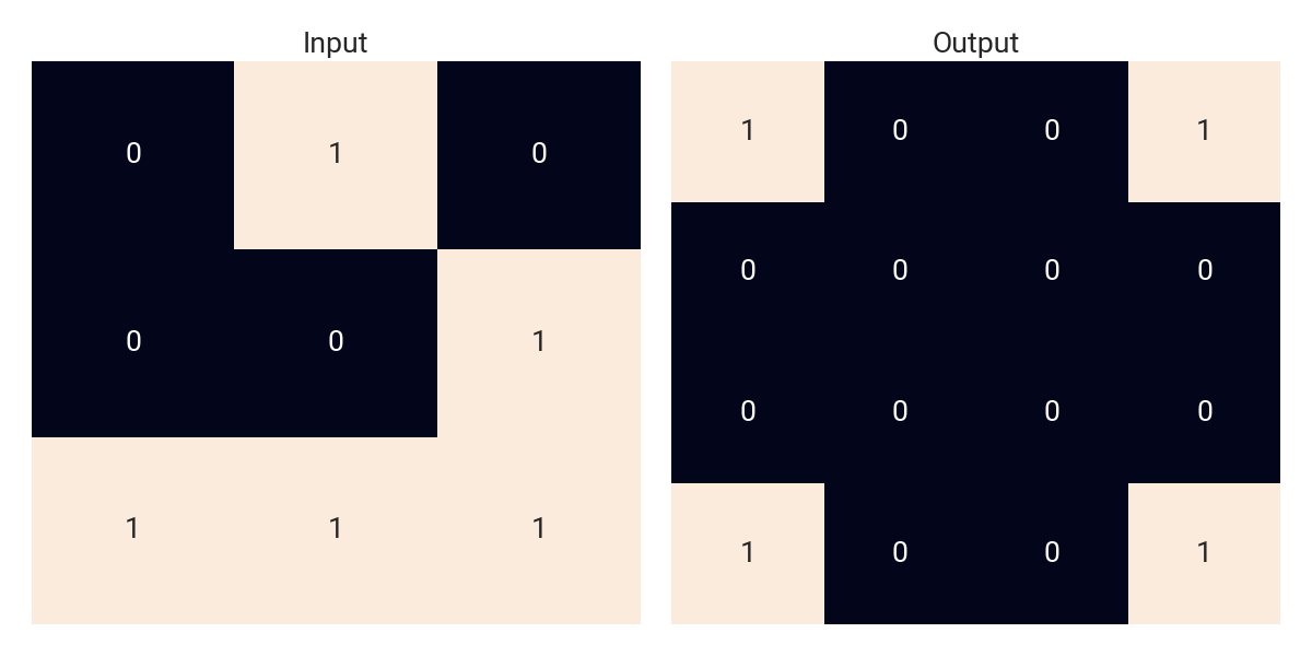
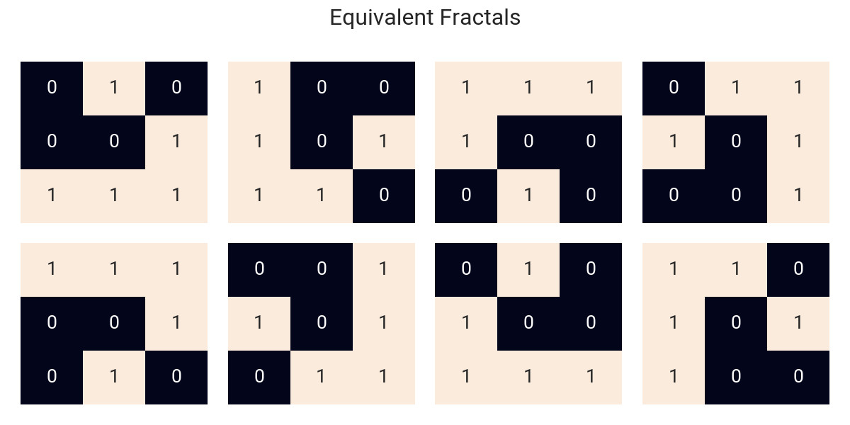
However, there’s a catch: not all possible input patterns are given. “Source” subgrids, hereinafter referred to as Fractals, are assumed to be invariant to mirroring (vertical and horizontal) and rotation (90°) operations, meaning that if one can be turned into the other via a sequence of these elemental operations, they are considered equal. For example, the following fractals are all equivalent inputs:
The result of the transformation, however, should remain as provided regardless of the transformations applied to the original pattern.
Given the rule-set, calculate how many #s will be in the grid after 5 and 18 iterations for parts 1 and 2 of the puzzle respectively.
Brute-Force: The Naïve Approach
Fractal Art falls into the category of AoC puzzles that provide explicit instructions on how to reach a solution. More often than not, this is an early warning that the direct implementation is computationally prohibitive. Nevertheless, for completeness’ sake I’ll go over it.
Naïve Representation
The first step is to parse the input. As a sequence of input/output pairs with distinct input fractals, it follows that the natural structure to store the rule-set is a hash-map. Since in Go, slices (i.e., arrays of unknown size) are not hashable, we can use the flattened pattern strings as keys and the expanded fractals as values. This is also why, despite the fractals assuming only one of two values for each of its slots, it is better to store the ASCII characters rather than converting them to booleans.
The above results in the following type definitions and function signatures (trivial implementations omitted):
type naiveFractal [][]byte
type naiveRuleset map[string]naiveFractal

func (f naiveFractal) serializeNaive() string
func deserializeNaive(serial string) naiveFractal

func initNaiveRuleset(lines []string) naiveRuleset {
 r := make(naiveRuleset)

 for _, line := range lines {
  kv := strings.Split(line, " => ")
  r[kv[0]] = deserializeNaive(kv[1])
 }

 return r
}
Naïve Matching
The next step is to match an incoming pattern with our rule-set. The simplest way to do so is to generate all equivalent fractals, which can be achieved by mirroring the fractal once (either vertically or horizontally) and then rotating both versions 3 times in the same direction (clockwise or anti-clockwise) for a total of 8 fractals, and checking their signatures (flattened string representation) in our rule-set. Since only one invariant per pattern is registered in the rule-set, the method should return the first match it encounters.
The above strategy is implemented in the transform function as follows:
func makeEmptyNaive(n int) naiveFractal

func (f naiveFractal) mirror() naiveFractal {
 n := len(f)
 fNew := make(naiveFractal, n)

 for i, row := range f {
  fNew[n-i-1] = slices.Clone(row)
 }

 return fNew
}

func (f naiveFractal) rotate() naiveFractal {
 n := len(f)

 fNew := makeEmptyNaive(n)

 for i := range n {
  for j := range n {
   fNew[i][j] = f[j][n-i-1]
  }
 }

 return fNew
}

func (r naiveRuleset) transform(f naiveFractal) naiveFractal {
 fm := f.mirror()

 for range 4 {
  if aux, ok := r[f.serializeNaive()]; ok {
   return aux
  }

  if aux, ok := r[fm.serializeNaive()]; ok {
   return aux
  }

  f = f.rotate()
  fm = fm.rotate()
 }

 panic("Unregistered source pattern: " + f.serializeNaive())
}
Sub-Indexing & Growth
We define a getter/setter pair that will allow us to query and modify square subregions from the grid; namely:
func (f naiveFractal) getSubfractal(i, j, n int) naiveFractal {
 subFractal := makeEmptyNaive(n)

 for k := range n {
  copy(subFractal[k], f[n*i+k][n*j:])
 }

 return subFractal
}

func (f *naiveFractal) setSubfractal(i, j, n int, sf naiveFractal) {
 for k := range n {
  copy((*f)[n*i+k][n*j:], sf[k])
 }
}
Here the main fractal is split into $n$-by-$n$ sub-fractals and select the $\left(i,j\right)$-th square. Then, since an iteration of the requested procedure increases the size of the grid deterministically, the resulting fractal can be pre-allocated and filled using the above helper methods. Thus, an iteration is implemented as follows:
func (r naiveRuleset) grow(f naiveFractal) naiveFractal {
 n := len(f)

 var s0, s1 int
 if n%2 == 0 {
  s0, s1 = 2, 3
 } else {
  s0, s1 = 3, 4
 }

 nSubfrac := n / s0
 fNext := makeEmptyNaive(nSubfrac * s1)

 for i := range nSubfrac {
  for j := range nSubfrac {
   fNext.setSubfractal(
    i, j, s1,
    r.transform(f.getSubfractal(i, j, s0)))
  }
 }

 return fNext
}
Putting it all together
Now all that’s left is to define the main callable. Nothing fancy; just an early return for the zero case, some initialization, and the main loop. To facilitate simultaneously testing multiple solutions, the Solver interface is also defined.
type Solver interface {
 String() string
 Solve(string, int, []string) uint
}

// Syntactic sugar to allow multiple implementations of the 'Solve' method
type NaiveSolver struct{}

func (s NaiveSolver) String() string { return "Naïve Solver" }

func (f naiveFractal) count() uint {
 var res uint

 for _, row := range f {
  for _, v := range row {
   if v == '#' {
    res++
   }
  }
 }

 return res
}

func (NaiveSolver) Solve(seed string, nIters int, lines []string) uint {
 if nIters == 0 {
  return uint(strings.Count(seed, "#"))
 }

 f := deserializeNaive(seed)
 r := initNaiveRuleset(lines)

 for range nIters {
  f = r.grow(f)
 }

 return f.count()
}
Great! Now, let’s loop over the number of iterations up to what was requested for part 2 and see how many does it take to get a good ol’ fatal error: runtime: out of memory:
goos: linux
goarch: amd64
pkg: github.com/sergiovaneg/GoStudy/AoC/2017/fractalArt
cpu: AMD Ryzen 5 5500U with Radeon Graphics
                           │   raw.txt   │
                           │   sec/op    │
Solvers/Naïve_Solver/0-12    6.740n ± 1%
Solvers/Naïve_Solver/1-12    62.64µ ± 1%
Solvers/Naïve_Solver/2-12    64.80µ ± 2%
Solvers/Naïve_Solver/3-12    70.16µ ± 2%
Solvers/Naïve_Solver/4-12    83.10µ ± 2%
Solvers/Naïve_Solver/5-12    111.4µ ± 1%
Solvers/Naïve_Solver/6-12    164.7µ ± 1%
Solvers/Naïve_Solver/7-12    257.5µ ± 1%
...
Solvers/Naïve_Solver/16-12   145.7m ± 2%
Solvers/Naïve_Solver/17-12   306.6m ± 2%
Solvers/Naïve_Solver/18-12   603.4m ± 3%
Huh…that’s odd. It works?
$\mathcal{O}(C^k)$, and how to Observe it
The naïve implementation turns out not to slow down as much as I expected for the second part, meaning that the grid size is still manageable; but just how big is it? Well, let $n_k$ be the side-length of the grid at iteration $k$; then, written as a recursion,
\[\begin{split} N_0 &= 3 \\ N_{k+1} &= \begin{cases} \frac{3}{2} \cdot N_k \quad & \text{if } N_k \text{ even} \\ \frac{4}{3} \cdot N_k \quad & \text{otherwise} \end{cases} \\ & \implies \left(\frac{4}{3} \right)^k \le \frac{N_k}{3} \le \left(\frac{3}{2} \right)^k \end{split}\]This means the grid grows exponentially, which entails $\mathcal{O}(C^k)$. If s alone aren’t scary enough, let’s take a look at some numbers:
| $k$ | $N_k$ | Size in Memory1 |
|---|---|---|
| 0 | 3 | 9 B |
| 1 | 4 | 16 B |
| 2 | 6 | 36 B |
| 3 | 9 | 81 B |
| 4 | 12 | 144 B |
| 5 | 18 | 324 B |
| 6 | 27 | 729 B |
| 7 | 36 | 1.27 KiB |
| 8 | 54 | 2.85 KiB |
| 9 | 81 | 6.41 KiB |
| $\vdots$ | $\vdots$ | $\vdots$ |
| 16 | 972 | 923 KiB |
| 17 | 1458 | 2.03 MiB |
| 18 | 2187 | 4.56 MiB |
So while in the first part we had to handle a 36B array, for part 2 we are allocating 4.5 MiB of memory, which is a million-plus-fold increase in the number of elements. But alas, inefficient as it is, computer hardware and compilers nowadays are good enough so that even my cheap-ass Huawei laptop can just brute-force a 2017 puzzle. Not just that, but the $1E6\times$ increase in size only incurred a $6E3\times$ increase in runtime.
For day 21, I was expecting the brute-force approach not to scale for part 2, and I admit I didn’t even try the naïve implementation until I started writing this blog. I guess problems back then didn’t blow up so spectacularly as the ones we’ve got in recent years (I’m looking at you specifically, Step Counter). Therefore, in order to observe a measurable effect as optimizations are introduced, let’s see how many iterations does it take to get to a nice round runtime; say, at least 10 seconds:
...
Solvers/Naïve_Solver/19-12    1.174 ± 1%
Solvers/Naïve_Solver/20-12    2.454 ± 2%
Solvers/Naïve_Solver/21-12    5.071 ± 2%
Solvers/Naïve_Solver/22-12    10.03 ± 2%
So 22 will be our target number of iterations. To avoid drowning this blog in logs, I will just show the benchmarks for 0, 1, 5, 18, and 22 iterations from now on. Don’t worry, I’ll draw some curves at the end to compare the performance gains from all
Brute-Force 2: Concurrent Boogaloo
First, I wanted to see how much of an improvement I could get out of Goroutines. It doesn’t matter what your stance is on Go or how verbose its error-handling is, one thing no one can deny is how ridiculously easy it is to refactor embarrasingly-parallel code and make it concurrent. For example, the grow method calls the transform function separately for each subregion of the grid; and since the next-generation grid is pre-allocated, making it concurrent requires little to no effort:
func (r naiveRuleset) growParallel(f naiveFractal) naiveFractal {
 n := len(f)

 var s0, s1 int
 if n%2 == 0 {
  s0, s1 = 2, 3
 } else {
  s0, s1 = 3, 4
 }

 nSubfrac := n / s0
 fNext := makeEmptyNaive(nSubfrac * s1)

 var wg sync.WaitGroup
 wg.Add(nSubfrac)
 for i := range nSubfrac {
  go func() {
   for j := range nSubfrac {
    fNext.setSubfractal(
     i, j, s1,
     r.transform(f.getSubfractal(i, j, s0)))
   }
   wg.Done()
  }()
 }
 wg.Wait()

 return fNext
}
So yeah, pretty much the same function with a wait-group in the middle. I decided to parallelize only the first iteration level for the sake of performance (more details in short). Now, let’s see some numbers:
                                      │    sec/op    │
Solvers/Naïve_Concurrent_Solver/0-12    6.813n ±  1%
Solvers/Naïve_Concurrent_Solver/1-12    61.82µ ±  3%
...
Solvers/Naïve_Concurrent_Solver/5-12    131.3µ ±  1%
...
Solvers/Naïve_Concurrent_Solver/18-12   160.8m ±  1%
...
Solvers/Naïve_Concurrent_Solver/22-12    2.034 ±  4%
So, a couple of things to highlight here:
- Green threads are cheap, but they’re not free. The cost of synchronization and spawning Goroutines makes it so that concurrency is initially as expensive as (or even more so than) single-threaded execution.
- As we increase the number of iterations, the improvement becomes clear, yielding a $5\times$ speed-up for 22 procedure iterations without modifying the algorithm or data structures.
Still, a pretty hefty improvement for what is essentially the same code. I wonder if there is another trivial optimization I might be missing…
Brute-Force 3: DP Rises
I’m not going to sit here and pretend Dynamic Programming is an inherently easy concept. In general, figuring what repeated calls to store without creating an infinite lookup table is a challenge on its own. However, the problem itself is giving us a bounded set of inputs we will ever have to calculate: the rule-set.
Since we will only ever need to transform fractals of size 2 and 3, assuming 1 of 2 values for each of its slots, we end up with a total of $2^4+2^9 = 528$ potential input fractals. Rather than transforming and matching the input pattern to its registered invariant as it is passed to the transform method, it is faster (at least in the long-term) to record them in the rule-set as-is.
Wouldn’t that be inefficient, though?
I mean, kinda? It ends up being around 5 times the original rule-set’s size, but we’re talking about 9-16 Byte fractals, so duplication is not that big of a deal. But alright: for the sake of memory efficiency, let us mod the rule-set a little:
type normalizer map[string]*string
type normalizedRuleset struct {
 r naiveRuleset
 n normalizer
}

func (nr normalizedRuleset) get(serial string) (naiveFractal, bool) {
 f, ok := nr.r[*nr.n[serial]]
 return f, ok
}
While it doesn’t seem like much of a change (and it practice it isn’t), we can effectively remove fractal duplication by creating an intermediate hash-map and making all equivalent serials point to the memory address of the registered one. In the case of $n=3 \rightarrow n=4$ transformations, we go from $8 \times 16B = 128$ Bytes to $8 \times 8B + 16B = 80$ Bytes per equivalent set. A fun little experiment that requires near-zero effort and yields near-zero gain.
Now, for the actual improvement, we have two ways of adding DP to the mix: tabulation and memoization. Both are relatively easy to implement through the current structures; however, if we want to preserve trivial concurrency, the rule-set hash-map cannot be modified while other threads are running, which is why I decided to stick to tabulation and pre-calculate the invariants during initialization. The resulting implementation is as follows (the grow method is just a copy of the growParallel method):
func initNormalizedRuleset(lines []string) normalizedRuleset {
 var nr normalizedRuleset
 nr.r = make(naiveRuleset)
 nr.n = make(normalizer)

 for _, line := range lines {
  kv := strings.Split(line, " => ")
  nr.r[kv[0]] = deserializeNaive(kv[1])

  f := deserializeNaive(kv[0])
  fm := f.mirror()

  for range 4 {
   s, sm := f.serializeNaive(), fm.serializeNaive()
   nr.n[s], nr.n[sm] = &kv[0], &kv[0]
   f, fm = f.rotate(), fm.rotate()
  }
 }

 return nr
}

func (nr normalizedRuleset) transform(f naiveFractal) naiveFractal {
 if out, ok := nr.get(f.serializeNaive()); ok {
  return out
 }

 panic("Unregistered source pattern: " + f.serializeNaive())

}

func (nr normalizedRuleset) grow(f naiveFractal) naiveFractal
So, with our new rule-set, we can go and see how much of an improvement we got:
                              │    sec/op    │
Solvers/Naïve_DP_Solver/0-12    6.495n ±  0%
Solvers/Naïve_DP_Solver/1-12    417.9µ ±  2%
...
Solvers/Naïve_DP_Solver/5-12    502.3µ ±  2%
...
Solvers/Naïve_DP_Solver/18-12   80.12m ±  9%
...
Solvers/Naïve_DP_Solver/22-12   711.2m ±  5%
It’s clear that, by using tabulation, we’re paying a heavier warm-up price. However, by the 18th iteration we have already got a return-on-investment, to the point where the 22nd iteration now is reachable in under a second. Considering we started at 10 seconds, this is a $14\times$ improvement without fundamentally changing the original algorithm, and a $3\times$ improvement over just concurrency.
However, not modifying the algorithm also means that its asymptotic complexity remains exponential. Well, what if I told you that by representing our state in a more clever way, focusing on what the problem is actually asking from us, it is possible to reach $\mathcal{O}(1)$ complexity?
Independent Evolution and Separable Elements
The original problem requests the number of # characters present after a number of iterations; it never says anything about their position. However, we have seen that fractals mix before applying the rules for every iteration, so it’s not as simple as applying the rules recursively for each sub-fractal. Thus, I decided to take a look at the behaviour of the algorithm during the first few iterations.
The Heuristic
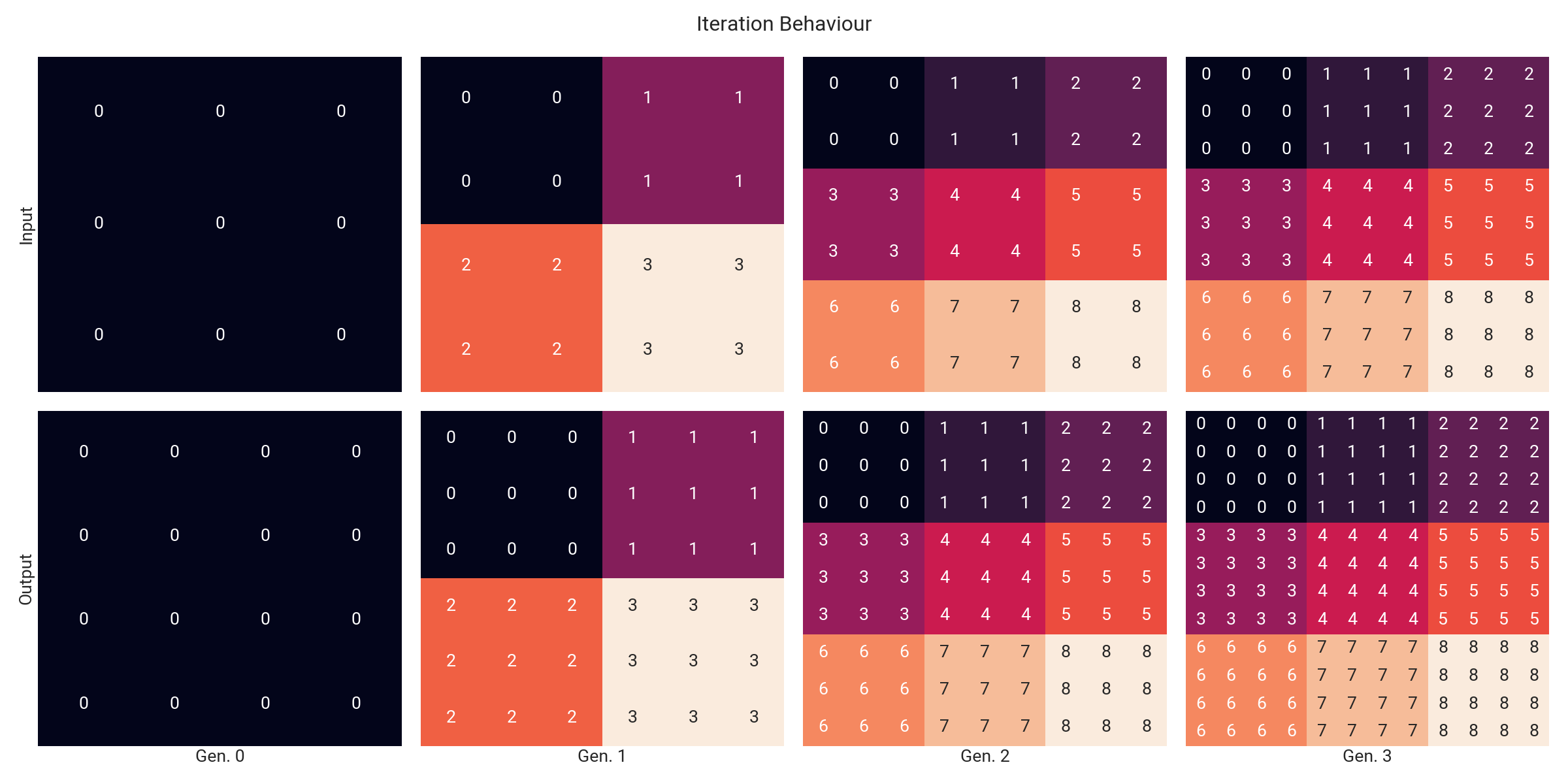
For each column, the colours and numbers above indicate the input-output subregion correspondence. Notice a pattern? There is a 3-periodic sequence in the algorithm; i.e., starting from a fractal of size $n=3$, after 3 iterations we get a set of 9 3-fractals that evolve independently and deterministically. This means that there is no need of tracking the position of these atomic elements with respect to each other, so we can just track the number of repeated normalized (since the first transition disregards orientation and mirroring) 3-fractals currently in our grid.
Keep in mind that whenever the requested number of iterations is not a multiple of 3, we will have to make the tracked elementary 3-fractals grow for the remaining number of generations. However, since they are already grouped, this procedure only has to be carried out once per distinct pattern. Finally, we can multiply the amount of # in the tracked sub-fractals by their number of instances and get the answer.
Since there are only $102$ unique normalized 3-fractals (according to the puzzle input), once $N_k \ge 3\sqrt{102}$ we are bound to have repeated patterns, which in our algorithm happens for the first time at $k=7$. This means that the cost of each iteration beyond this point (or even earlier if the seed/rule-set pair is such that some 3-fractals never show up in the sequence) becomes constant. Moreover, the cost of iterating can be further reduced by applying some of the optimizations we have reviewed so far to this new macro-loop.
The Implementation
First, we define some new data structures:
type stateSequence struct {
 s1, s2 string
 s3     map[string]uint
}
type stateRuleset map[string]state
type groupedRuleset struct {
 rules      normalizedRuleset
 stateRules stateRuleset
}
Here, stateSequence is a structure that stores the 3 states generated by a (normalized) 3-fractal:
s1, the serial of the 4-fractal associated to the normalized serial in the original rule-set;s2, the serial of the 6-fractal following the above 4-fractal;- and
s3, a hash-map giving the frequency of the 9 3-fractals forming the 9-fractal at the end of the 3-step sequence.
Then, stateRuleset memoizes previously observed 3-step transitions indexed by the normalized 3-fractal serial. Finally, groupedRuleset is naught but syntactic sugar to pass both the single-step normalized rule-set and the new 3-step rule-set as a single argument.
Now, we move onto the heart of the algorithm: we exploit the previously-defined methods to go from a 3-fractal to a 9-fractal deterministically, followed by an extraction of the 9 3-fractals that described to successive state, recording the transition in the state rule-set. That way, every time growThrice is called, the transition will be registered if not present and then returned.
func (gr *groupedRuleset) updateSR(serial string) {
 f0 := deserializeNaive(serial)

 var f1 naiveFractal
 s := stateSequence{
  s3: make(map[string]uint),
 }

 // 3x3 -> 4x4
 f0 = gr.rules.transform(f0)
 s.s1 = f0.serializeNaive()

 // 4x4 -> 6x6
 f1 = makeEmptyNaive(6)
 for i := range 2 {
  for j := range 2 {
   subFractal := f0.getSubfractal(i, j, 2)
   subFractal = gr.rules.transform(subFractal)
   f1.setSubfractal(i, j, 3, subFractal)
  }
 }
 f0 = f1
 s.s2 = f0.serializeNaive()

 // 6x6 -> 9x9
 f1 = makeEmptyNaive(9)
 for i := range 3 {
  for j := range 3 {
   subFractal := f0.getSubfractal(i, j, 2)
   subFractal = gr.rules.transform(subFractal)
   f1.setSubfractal(i, j, 3, subFractal)
  }
 }
 f0 = f1

 // 9x9 -> 9 * 3x3
 for i := range 3 {
  for j := range 3 {
   subfractal := f0.getSubfractal(i, j, 3)
   normSerial := *gr.rules.n[subfractal.serializeNaive()]
   s.s3[normSerial]++
  }
 }

 gr.stateRules[serial] = s
}

func (gr *groupedRuleset) growThrice(serial string) stateSequence {

 if _, ok := gr.stateRules[serial]; !ok {
  gr.updateSR(serial)
 }

 return gr.stateRules[serial]
}
Finally, we exploit this new method and the earlier ones to implement the Solve method:
func initGR(lines []string) groupedRuleset // Trivial, thus omitted

func (GroupedSolver) Solve(seed string, nIters int, lines []string) uint {
 if len(seed) != 11 {
  panic("Invalid seed: serial should match a 3x3 fractal.")
 }

 if nIters == 0 {
  return uint(strings.Count(seed, "#"))
 }

 gr := initGR(lines)

 // Normalize from the beginning
 state0 := map[string]uint{*gr.rules.n[seed]: 1}

 for range nIters / 3 {
  state1 := make(map[string]uint)

  for serial0, cnt0 := range state0 {
   for serial1, cnt1 := range gr.growThrice(serial0).s3 {
    state1[serial1] += cnt0 * cnt1
   }
  }

  state0 = state1
 }

 var finalCount uint

 switch nIters % 3 {
 case 0:
  for serial, cnt := range state0 {
   finalCount += cnt * uint(strings.Count(serial, "#"))
  }
 case 1:
  for serial, cnt := range state0 {
   finalCount += cnt * uint(strings.Count(
    gr.growThrice(serial).s1, "#"))
  }
 case 2:
  for serial, cnt := range state0 {
   finalCount += cnt * uint(strings.Count(
    gr.growThrice(serial).s2, "#"))
  }
 }

 return finalCount
}
Note that concurrency was not used this time, since the overhead from aggregating up to 102 maps for what is essentially a retrieval-by-key is simply not justified.
The Numbers
                             │   sec/op    │
Solvers/Grouped_Solver/0-12    7.401n ± 2%
Solvers/Grouped_Solver/1-12    420.6µ ± 1%
Solvers/Grouped_Solver/2-12    425.7µ ± 2%
Solvers/Grouped_Solver/3-12    424.6µ ± 1%
Solvers/Grouped_Solver/4-12    453.3µ ± 2%
Solvers/Grouped_Solver/5-12    461.0µ ± 2%
Solvers/Grouped_Solver/6-12    452.3µ ± 2%
Solvers/Grouped_Solver/7-12    457.5µ ± 1%
Solvers/Grouped_Solver/8-12    455.0µ ± 2%
Solvers/Grouped_Solver/9-12    458.1µ ± 4%
Solvers/Grouped_Solver/10-12   462.6µ ± 1%
Solvers/Grouped_Solver/11-12   470.9µ ± 2%
Solvers/Grouped_Solver/12-12   457.8µ ± 2%
Solvers/Grouped_Solver/13-12   459.6µ ± 4%
Solvers/Grouped_Solver/14-12   460.9µ ± 2%
Solvers/Grouped_Solver/15-12   465.9µ ± 2%
Solvers/Grouped_Solver/16-12   463.7µ ± 1%
Solvers/Grouped_Solver/17-12   466.9µ ± 1%
Solvers/Grouped_Solver/18-12   468.4µ ± 3%
Solvers/Grouped_Solver/19-12   466.2µ ± 4%
Solvers/Grouped_Solver/20-12   463.6µ ± 3%
Solvers/Grouped_Solver/21-12   472.6µ ± 3%
Solvers/Grouped_Solver/22-12   468.5µ ± 3%
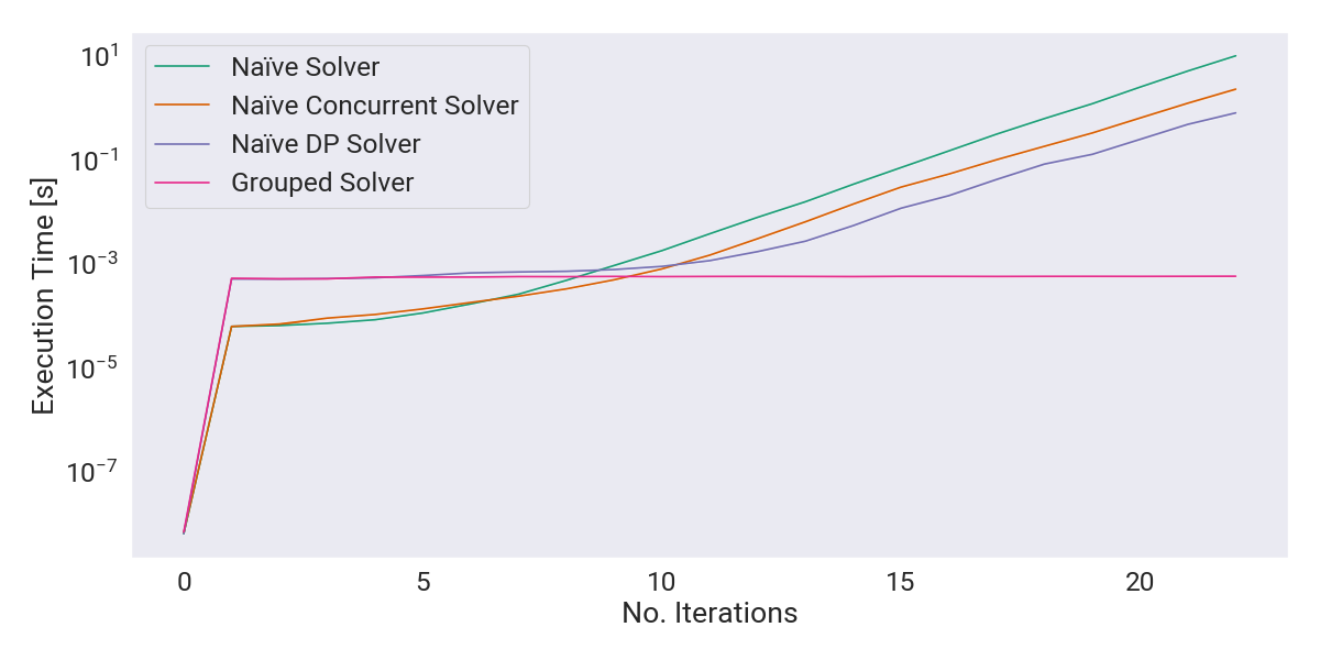
This time, I left all the results to confirm my earlier hypothesis: as predicted, after the sixth iteration, the algorithm is just retrieving transitions from the memoization table, which henceforth results in near-constant time.
Wrapping Up
All the code implementing the described solutions, as well as the test suite and the figure-generation script, can be found in my Codeberg repo.
Further optimizations could be made by exploiting the predetermined shapes in the 3-step sequences, using fixed-size arrays (or even bit-masks) instead of slices and strings to represent the state of the system. Moreover, as I mentioned earlier, there is performance left on the table due to Go being a garbage-collected programming language. Perhaps I’ll revisit this problem and extend the results once Zig reaches 1.0, and continue from this last implementation.
Regardless, I’m satisfied with how intuitive this heuristic was for me, and I hope this wasn’t just a fluke. I will try to do a similar write-up for other problems I find interesting, perhaps using Elixir or trying OCaml instead. For the time being, I should probably go back to work and check how the hyperparameter search is going 🫠.
-
Not the exact size in memory, since dynamic arrays (Slices) also store their length and each row is stored as a pointer. Nevertheless, the effect is negligible. ↩